Transaction Tables (Godley Tables)
Godley Tables
A simple transaction table for Private Banks:
| Flows↓/Stock Vars → | Reserves | Households | Firms | Equity | BanksEquity | A-L-E |
|---|---|---|---|---|---|---|
| Initial Conditions | 100 | 20 | 70 | 10 | 0 | 0 |
| Pay Wages | 0 | Wages | -Wages | 0 | 0 | 0 |
| Consumption | 0 | -Consume | Consume | 0 | 0 | 0 |
| ∫ Flows | 100+∫(flows) | 20+∫(flows) | 70+∫(flows) | 10+∫(flows) | 0 | 0 |
The bottom row shows the accumulation of flow transactions over time, this is the value of the stock at any time. The calculation is done at each time step by calculating the sum of all the flow values in that column, and than adding the sum to the current value of the stock. This can be likened to a number of pipes flows of water into a tank, the tank accumulates or integrates all the flows over time. Banks will do this accumulation step once every day.
Rate of Change or Differential Equations
The rate of change of each stock is the symbolic sum of the relevant column:
\[\frac{dFirms}{dt} = Consume - Wages\]
\[\frac{dHouseholds}{dt} = Wages - Consume\]
\[\frac{dFirms_{Equity}}{dt} = Consume - Wages \quad (2)\]
\[\frac{dHH_{Equity}}{dt} = Wages - Consume\]
\[\frac{dBanks_{Equity}}{dt} = 0\]
\[\frac{dReserves}{dt} = 0\]
\[\frac{dCB_{Equity}}{dt} = 0\]
These equations can be implemented in CircuitJS using Godly Tables, consisting of Flows on the rows, Stocks on the columns. The bottom row value is the integration of all the flows of that column.
This makes it possible to develop economic models with these tables, by defining these flows in terms of each other and relevant parameters. Here we implement this in CircuitJS, using the same approach as Matlab does with Simulink: flowcharts are used to generate equations for numerical simulation. The circuit to the left implements the following equations
Parameters and Flows
\[Wage_{share} = 0.6; \quad V_{Firms} = 2; \quad V_{HH} = 4\]
\[GDP = {Firms} \times {V_{Firms}}\]
\[Wages = GDP \times Wage_{share}\]
\[Consume = {Households} \times {V_{HH}} \quad (3)\]
\[Credit = GDP \times Credit_{share}\]
\[Interest = Debt_{Firms} \times Int_{rate}\]
\(V_{Firms}\) and \(V_{HH}\) is the velocity or rate of firms and householders money spending, the rate at which their money is exchanged in one year.
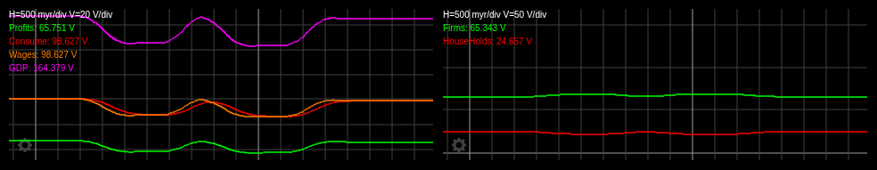
Note that in this economics system there is no money creation or credit. The existing money is merely moved around and the total sum of money remains the same at $100 with only $90 in the economy at one time, with wages and consumption flows at ~ $83 per yr.
Adjusting the slider for the Firms spend rate \(V_{Firms}\) will change the allocation of money and GDP.
| Variable | Value |
|---|---|
| Loading… | — |
This system is sustainable with only private sector debt.
| ← Prev | Next: Two Competing Models of Banking → |